
8. Downstream analysis#
After aggregating, profiles are typically processed before being used for analysis purposes. Data-processing approaches for profiles extracted with CellProfiler were described in the paper “Data analysis strategies for image-based profiling”. Some of those approaches were used for features extracted with DeepProfiler.
8.1 Aggregating and evaluating profiles with profiling notebooks#
To analyse benchmark datasets analysis paper we created
Jupyter notebooks, which are available in DeepProfilerExperiments Github repository.
Folders ta-orf (BBBC037 dataset), bbbc022 and cdrp (BBBC036 dataset) correspond to benchmark datasets and contain
Jupyter notebooks, profiling folder contains utility functions. Next, we are going to go through the most important
analysis notebooks. You can reuse this code to build a custom analysis pipeline.
8.1.1 Aggregation of profiles and batch-correction#
Aggregation of features can be done with 01-create-profiles.ipynb
Jupyter notebook. The inputs are: project metadata file, ground truth metadata
with annotations of treatments by the mechanism of action and the .npz files with features organized in
{Plate}/{Well}/{Site}.npz folder structure.
Define the parameters: project path and experiment folder name as in DeepProfiler, sphering regularization parameter
REG_PARAMand output file names:OUTPUT_FILE- output file that will contain well-level profiles after sphering andMATRIX_FILEthat will contain similarity matrix of treatments.Load single-cell data by passing through metadata and reading files with features. It might require a significant amount of RAM (depending on the size of the dataset).
Aggregate features of single-cells by site with median aggregation.
sitesPandas dataframe will contain those aggregated profiles.Aggregate site-level profiles to well-level using mean aggregation and store them in
wellsdataframe.Sphering: calculate the sphering transformation using control wells only and then apply this transformation to all well-level profiles in
wells.Aggregate well-level profiles to treatment-level profiles. Only treatments with ground truth annotations are aggregated and stored in
profilesdataframe.Create a similarity matrix from
profiles. We use cosine similarity as a similarity metric. Save the matrix toOUTPUT_FILE.
8.1.2 Batch-correction using sphering transformation#
The sphering transformation (implementation) aims to reduce unwanted technical variation and recover the phenotypic features of treatments from the latent representations of the weakly supervised CNN. We calculate the ZCA-transformation matrix using well-level profiles of negative controls. The assumption here is that phenotypic features of negative controls should be neutral, thus the difference between them encodes mostly technical and irrelevant variation.
Sphering transformation can be regularized, the strength of regularization is regulated by REG_PARAM in the notebook,
a good value to start is 1e-3, though it depends on the data.
The calсulated ZCA-transformation matrix is used to calculate corrected profiles (both for treated wells and control wells). On the UMAP plot, negative control wells are expected to group, and treated wells with relatively weak phenotypes are also expected to group with negative control wells.
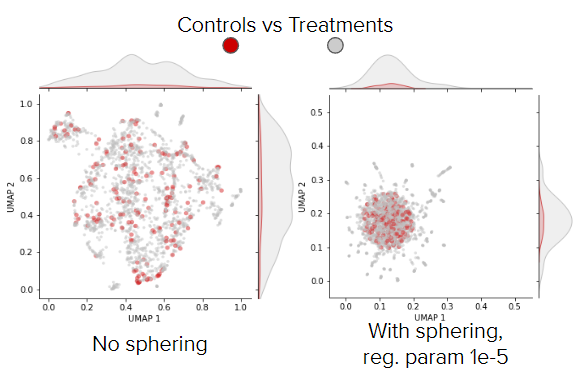
Fig. 10 UMAP of well-level profiles before and after sphering (BBBC037 dataset). Red point are control wells, gray points are treated wells and blue points are treatments.#
8.1.3 Evaluation of profiles#
Evaluation of profiles can be done with 04-downstream-analysis.ipynb. This notebook uses the cosine similarity matrix
obtained in 01-create-profiles.ipynb as an input.
First parts (Load similarity matrix and MOA matching) of the notebook perform input pre-processing.
moa_matchesis a binary matrix of sizen x n, wherenis the number of treatments in the similarity matrix. This matrix is symmetrical and each row (column) relates is a treatment, and values areTruein each row (column) for the current treatment (diagonal) and treatments that belong to the same mechanism of action as the current treatment.Calculate the precision metrics:
Average precisionandPrecision @ top 1%.Calculate the recall metrics:
RecallandAverage Recall at top 10%(a different cut-off was used on purpose).Calculate mean Average Precision, and area under interpolated Precision-Recall curve and plot it.
Save results to the
.csvtable andpickle(contains Python dictionary and can be loaded with Python).
8.1.4 Visualize profiles#
The visualizations can be done with 02-profiles-visualizations.ipynb
Jupyter notebook. The input is a path to well-level profiles and is set in INPUT_PROFILES.
Treatment-level profiles are calculated using mean aggregation.
The UMAP transformation is obtained using only well-level profiles. Get embeddings for well-level profiles.
Use transformation from the previous step for treatment level profiles.
Plot embeddings both from well and treatment-level profiles (see below).
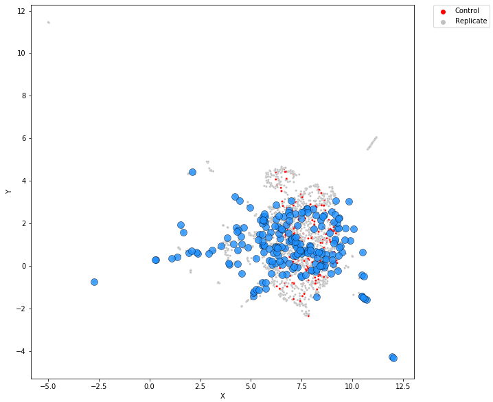
Fig. 11 Example of visualization (BBBC037 dataset).#
8.2 Aggregating and evaluating profiles with Pycytominer#
DeepProfiler single-cell profiles can be aggregated via a Pycytominer function called DeepProfiler_Processing. This function reads the output features of DeepProfiler, including the metadata, aggregates, and saves the data in a Pycytominer and Cytominer-eval readable data frame format.
Make sure to install this version of Pycytominer:
pip install git+git://github.com/cytomining/pycytominer@update_agg_TF2
This code gives an example of how to run the aggregation function:
import os
import numpy as np
import pandas as pd

from pycytominer.cyto_utils.DeepProfiler_processing import AggregateDeepProfiler

project_dir = os.path.join(
    os.path.dirname(__file__)
)

experiment = 'folder_name'

profile_dir = os.path.join(project_dir, "outputs", experiment, "features")

metadata_file = os.path.join(project_dir, "inputs", "metadata", "index.csv")

output_folder = os.path.join(project_dir, 'outputs',experiment,'aggregated')

well_class = AggregateDeepProfiler(
    metadata_file=metadata_file,
    profile_dir=profile_dir,
    aggregate_operation="median",
    aggregate_on="well",
    output_file=output_folder,
)
df_well = well_class.aggregate_deep()

df_well.to_csv('aggregated_efficientnet_median.csv')
The Cytominer-eval repository contains six functions that calculate different quality metrics for perturbation profiling experiments: Precision@K and Recall@K, Enrichment, Hit@k, Replicate reproducibility, MP-value, and Grit.